11/5/2026
Data ScienceCentral Limit Theorem: Why Sample Means Form a Bell Curve
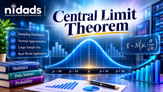
Table of contents
Central Limit Theorem: How Repeated Samples Reveal a Bell Curve—and Why It Matters for Statistical Inference
What Is the Central Limit Theorem?
Draw a lot of random samples, all the same size, and average each one. Plot those averages and you get an approximately normal, bell-shaped curve. That’s the Central Limit Theorem (CLT). It works even if the raw data is skewed, as long as observations are independent, the variance is finite and the sample is big enough. The payoff is practical: you can build confidence intervals and run hypothesis tests on a population mean without needing normally distributed raw data.
Key Takeaways
- The CLT is about sample means, not raw data.
- The population doesn’t have to be normal.
- Standard error is σ/√n, so it shrinks as n grows.
- A bigger n helps, but n ≥ 30 is just a rule of thumb.
- Samples must be random and independent, with finite variance.
- Confidence intervals and many common tests lean on it.
Core Idea in Simple Words
Averages are calmer than single values. Picture daily rainfall: a handful of storm days and the whole dataset looks lopsided. Now grab 40 random days and average them. Do it again. And again. The averages pile up into a bell shape, since the storm days in one sample get offset by the dry days sitting next to them.
That pile of averages has a name: the sampling distribution of the sample mean. The CLT is about that, not the raw data. It’s one of the most useful statistical concepts in data science, mostly because almost everything you report is some kind of average. [add your own line]
The Formula
Take independent, identically distributed observations with a finite mean μ and a finite, non-zero variance σ². Then:
(X̄ − μ)/(σ/√n) approaches N(0,1) as n grows.
In day-to-day use you’ll see it written as X̄ ≈ N(μ, σ²/n).
- X̄ is the sample mean, μ the population mean, n the sample size.
- σ measures the spread of single values.
- σ/√n is the standard error, the spread of sample averages.
- N(0,1) is the standard normal curve.
If the notation feels rusty, a quick look at probability and statistics for data science will sort it out.
A side note. Usually you don’t know the population standard deviation, so inference about the mean uses the sample standard deviation s and a t procedure. That procedure is exactly valid in small samples only when the observations are normal. With non-normal data, check your sample size and the shape of the data before trusting it.
How It Works, Step by Step
- Define the population and its mean.
- Draw a random sample of size n.
- Calculate the sample mean.
- Repeat many times, in theory or by simulation.
- Plot the means. A bell appears, centered at μ, with spread σ/√n.
| Term | Meaning |
| Population | Everything you want to study |
| Sample | The part you actually observe |
| Sampling distribution | How the sample mean varies from sample to sample |
Practical Examples (Hypothetical)
Example 1: A probability. Delivery times have μ = 40 minutes and σ = 10 minutes. You sample n = 25 deliveries. What’s P(sample mean > 43)?
- SE = 10/√25 = 2
- z = (43 − 40)/2 = 1.5
- P(Z > 1.5) = 1 − 0.9332 = 0.0668
What it means: if the true mean really is 40, about 6.7% of samples like this would average above 43. It’s a normal-approximation estimate, though. Delivery times are usually skewed, so the true probability depends on their actual distribution. A quick simulation will tell you.
Example 2: A confidence interval. A machine fills packages with σ = 4 g. A random sample of n = 64 packages averages 101.2 g.
- SE = 4/√64 = 0.5
- 95% interval = 101.2 ± 1.96 × 0.5 = 101.2 ± 0.98
- Result: 100.22 g to 102.18 g
What it means: the true average plausibly falls in that range, assuming the sample is random and independent.
Lesson: divide by the standard error, not σ.
Original Framework: The SAFE Check
This is a memory aid I use, not a formal standard. It helps you decide whether a normal approximation is reasonable:
- Sampling is random and unbiased.
- All observations are independent, with no clusters and no time order.
- Finite variance. Extreme outliers don’t break the CLT, but they slow convergence, so dig into them.
- Enough n for the data’s skew. Plot it, or simulate.
 When one of these fails, the fix is a better study design. Bias and dependence don’t vanish by themselves. A bootstrap only helps if its resampling matches the data, and a larger n will never cure bias.
Why 30 isn’t magic: take a very skewed distribution like the exponential. Its sample means still have skewness near 0.37 at n = 30. Heavy-tailed data can stay far from normal at much larger sizes.
Comparison: CLT vs Law of Large Numbers vs Normal Distribution
| CLT | Law of Large Numbers | Normal distribution | |
| What it is | A theorem about the shape of sample means | A theorem about where sample means end up | A specific bell-curve distribution |
| Says | Means become approximately normal | Means approach μ | Describes a symmetric variable |
| Use | Confidence intervals, tests | Justifies estimation | Modeling and probabilities |
The law of large numbers doesn’t make raw data normal. To see how the normal curve compares with other probability distributions and statistical analysis methods, test them side by side on real data.
Use Cases, Tools, Benefits and Limits
Use cases: surveys, A/B tests, quality control charts, machine learning evaluation and business reporting.
Tools: Python (NumPy, Matplotlib), R and Excel.
python
import numpy as np
import matplotlib.pyplot as plt
rng = np.random.default_rng(42)
fig, axes = plt.subplots(1, 3, figsize=(12, 3.5))
for ax, n in zip(axes, [5, 30, 200]):
means = rng.exponential(1, (10000, n)).mean(axis=1)
ax.hist(means, bins=40)
ax.set_title(f"Sample size n = {n}")
ax.set_xlabel("Sample mean")
ax.set_ylabel("Frequency")
plt.tight_layout()
plt.show()
For each n, this draws 10,000 samples from a skewed exponential population. At n = 5 the histogram leans heavily to one side. At n = 30 it starts to look like a bell. By n = 200 it’s narrow and nearly symmetric. The center stays near 1 and the spread shrinks like 1/√n. One caution: a simulation illustrates the theorem, it doesn’t prove it.
Benefits: simple, fast, and it works for a wide range of populations.
Limits: it’s only an approximation. Small n, heavy tails (the Cauchy, for example) and dependent data all give it trouble.
Best Practices and Common Mistakes
Do: plot your data first. Report the standard error or a confidence interval. When σ is unknown, check the shape of the data. And be upfront that results are approximate. [add your own line]
Avoid:
- Using σ instead of σ/√n for averages.
- Believing n = 30 always works.
- Thinking the raw data become normal.
- Assuming a bigger sample removes bias.
Practice questions:
- If μ = 200, σ = 30 and n = 100, what’s the standard error? Answer: 30/√100 = 3.
- Find P(sample mean > 206) for the same data. Answer: z = (206 − 200)/3 = 2, so P = 1 − 0.9772 = 0.0228.
- What happens to SE when n is multiplied by 4? Answer: it’s cut in half.
Evidence and Trusted Sources
The standard error and sampling distribution explanations here match the OpenStax Introductory Statistics chapter on the central limit theorem, a free university-level textbook.
For confidence intervals and t procedures, see the NIST/SEMATECH e-Handbook of Statistical Methods, a trusted government reference.
Related Questions and FAQs
1. What is the central limit theorem in simple words?
As samples grow, their averages form a bell curve, even if the data itself isn’t bell-shaped.
2. What is the central limit theorem formula?
(X̄ − μ)/(σ/√n) approaches N(0,1). In practice, X̄ ≈ N(μ, σ²/n).
3. Why is the central limit theorem important?
It lets us build confidence intervals and tests for means without needing normal raw data.
4. What sample size does the CLT need?
It depends. n ≥ 30 is a rough guide, but skewed or heavy-tailed data can need far more.
5. Does the population have to be normal?
No. Only the distribution of sample means becomes approximately normal.
6. CLT vs law of large numbers: what’s the difference?
The law says the sample mean gets close to μ. The CLT describes the bell-shaped spread around μ.
7. What is standard error?
The standard deviation of the sample mean, σ/√n. With σ = 12 and n = 36, it’s 2.
8. How do you show the CLT in Python?
Sample a skewed distribution many times, average each sample and plot the means (see the code above).
Conclusion
The Central Limit Theorem is the reason averages behave more predictably than single values. Repeated random samples give sample means that form a bell curve around the true population mean, with a spread equal to the standard error, sigma divided by the square root of n. Before you trust the approximation, check independence, finite variance and sample size. Then run the Python simulation with n = 5, 30 and 200 and solve the practice problems yourself. That’s what makes it stick.